GDPR is now in effect in Europe and you are still wondering how you are going to handle this? No worries, MongoDB Views are here to help but first a little definition.

Definition

“Pseudonymization is a data management procedure by which personally identifiable information fields within a data record are replaced by one or more artificial identifiers, or pseudonyms. A single pseudonym for each replaced field or collection of replaced fields makes the data record less identifiable while remaining suitable for data analysis and data processing.”

MongoDB Views

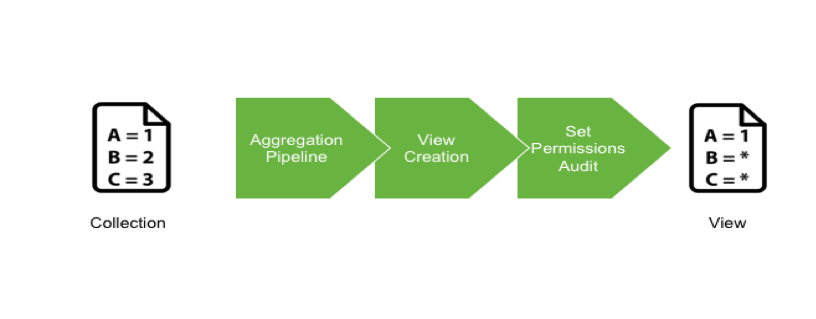
A view in MongoDB is a read-only projection of an existing collection or another view. The purpose of a view is to provide an alternative way to present documents. As we use the Aggregation Pipeline to generate a view, a projection can be done to pseudonymize each field. Consequently, it is possible to create several views, based on use cases and keep a golden copy of the data on the Master Collection.

Considerations

• Views are read only
• Views use index from the master collection
• Some restrictions exist for the projection - see Official MongoDB Documentation

Example

I want to show you a practical approach to pseudonymization using views in MongoDB. We will be using a Game of Thrones characters collection, with their status (dead/alive). Here is an example of one document:

{
    "_id" : ObjectId("5ae13de5f54a365254c62ad1"),
    "firstName" : "Daenerys",
    "lastName" : "Targaryen",
    "nickName" : "Khaleesi",
    "house" : "Targaryen",
    "actor" : "Emilia Clarke",
    "gender" : "female",
    "status" : "alive"
}


You can download the dataset here.

And you can import it directly from command line:

mongoimport --drop -d gameofthrones -c characters 
gameofthrones.characters.json


Explore the dataset and notice that the “status” is not always specified. Sometimes this key/value is missing and we need to take that into account in our view.

Because the “status” is a sensitive data full of spoilers, we want to hide this in a spoiler-free view.

Create the view

In this example, we used the following aggregation pipeline to generate the view:

> use gameofthrones
> db.characters.aggregate([
{ "$project" : 
    { 
        _id : 0,
        "firstName" : 1, 
        "lastName" : 1, 
        "house" : 1,
        "status" : 
        {
            "$cond": [{ "$eq": [ "$status", undefined ] }, $status = "Not Specified", $status = "*****" ],
        }    
    } 
} 
])


This aggregation pipeline will project the collection and replace the content of the field “status” with “*****” if this field exists. If not, the “status” will mention “Not Specified”.

Let’s create a view called “charactersNoSpoil”, based on the “characters” collection. We can leverage the aggregation pipeline created in the previous step:

> use gameofthrones
> db.createView(
  "charactersNoSpoil", 
  "characters", 
  [{ 
     "$project" : 
       { 
         _id : 0,
         "firstName" : 1, 
         "lastName" : 1, 
         "house" : 1, 
         "status" : 
           {"$cond": [{ "$eq": [ "$status", undefined ] }, $status = "Not Specified", $status = "*****" ]}
        }
  }] 
)


With the view created you can check it by performing a “show collections”, a “db.getCollectionInfos()” or a “db.charactersNoSpoil.find()” command.

> use gameofthrones
> db.charactersNoSpoil.find({},{firstName:1, status:1})
{ "firstName" : "Daenerys", "status" : "*****" }
{ "firstName" : "Joffrey", "status" : "*****" }
{ "firstName" : "Robert", "status" : "*****" }
{ "firstName" : "Tyron", "status" : "Not Specified" }
{ "firstName" : "Jaime", "status" : "*****" }
{ "firstName" : "Jon", "status" : "*****" }
{ "firstName" : "Cersei", "status" : "*****" }
{ "firstName" : "Sansa", "status" : "*****" }
{ "firstName" : "Tywin", "status" : "Not Specified" }
{ "firstName" : "Arya", "status" : "Not Specified" }
{ "firstName" : "Eddard", "status" : "Not Specified" }


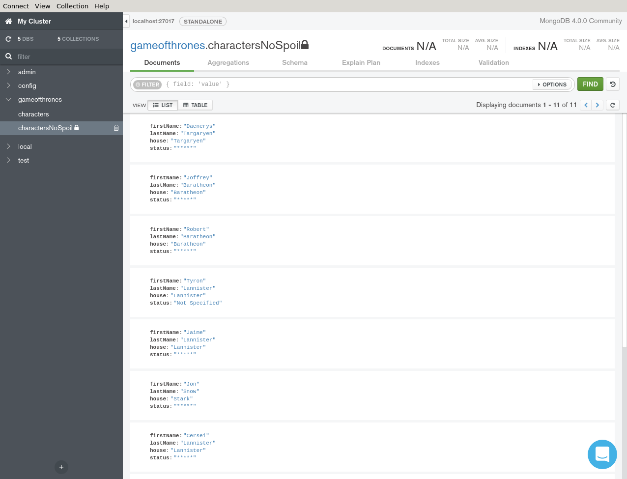
If you are using MongoDB Compass, you should see the following result.

Working with Views

As mentioned in the introduction, views are read-only and use the index from the collection source.

Insert a new document

To add a new document on the view, you have to create the document on the original collection. The new document will be automatically accessible through the view.

> db.characters.insertOne({
  "firstName": "Hodor", 
  "actor": "Kristian Nairn", 
  "gender": "male", 
  "status": "dead"
})


Then check that this document appears within the “charactersNoSpoil” view.

> db.charactersNoSpoil.find({firstName: "Hodor"}) 
{ "firstName" : "Hodor", "status" : "*****" }


Create an Index

To create an index that could be used by the view, you have to create an index on the collection.

> db.characters.createIndex({"house":1})
> db.charactersNoSpoil.find({house: "Stark"}).explain()

extract of the winning plan:
"winningPlan" : {
    "stage" : "FETCH",
    "inputStage" : {
        "stage" : "IXSCAN",
        "keyPattern" : {"house" : 1},
        "indexName" : "house_1",
        "isMultiKey" : false,
        "multiKeyPaths" : {"house" : [ ]},
        "isUnique" : false,
        "isSparse" : false,
        "isPartial" : false,
        "indexVersion" : 2,
        "direction" : "forward",
        "indexBounds" : {"house" : ["[\"Stark\", \"Stark\"]"]}
    }
}


And as you can see here the explain plan shows we are using the index {“house”:1} for the find in our view.

Setup the Access control

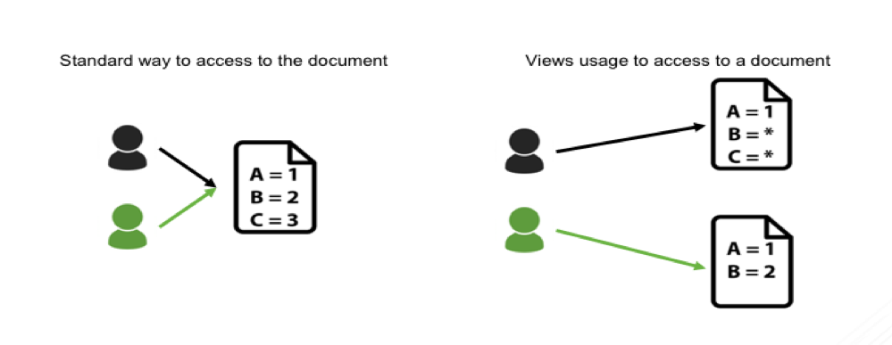
Now that the view is created, it is important to segregate who can read the view and who can write to the master collection.

To enforce this example, you will create users and roles to secure the data.

• Alice should only be able to write in the master collection,
• Bob should only be able to read the view.

By doing this, you will prevent unauthorized read to the “characters” collection, thus no spoilers :-).

Before starting

If you have not done that already, you need to enable Role-Based Access Control on your MongoDB server by adding “--auth” in the command line or by adding the following lines into your “/etc/mongod.conf” file.

security:
 authorization: enabled


Then you need to connect, create an admin user and log in as this new admin user.

> use admin
> db.createUser( { user: "admin", pwd: "safepassword", roles:["root"] })
> db.auth("admin","safepassword")


If you want to know more about our security recommendations for running MongoDB in production, have a look at our security checklist.

Create the roles

Now that we have a super user, we can create the two roles we need for Alice and Bob.

The first role “writeOnly” will be for Alice:

> use admin
> db.createRole({
    role  : "writeOnly",
    privileges : [
      {
        resource : { db : "gameofthrones", collection : "characters" },
        actions  : [ "insert" ]
      }
    ],
      roles : []
    })


And the second one for Bob:

> use admin
> db.createRole({
    role  : "noSpoilers",
    privileges : [
      {
        resource : { db : "gameofthrones", collection : "charactersNoSpoil" },
        actions  : [ "find" ]
      }
    ],
      roles : []
    })


Now we can create our two users:

> use admin
> db.createUser({ user : "Alice", pwd : "a", roles : ["writeOnly"] })
> db.createUser({ user : "Bob", pwd : "b", roles : ["noSpoilers"] })


Verifications

Alice has only been granted the right to insert into the collection “characters”.

$ mongo -u Alice -p a --authenticationDatabase admin gameofthrones
> db.characters.insertOne({
  "firstName": "Catelyn", 
  "lastName": "Stark", 
  "actor": "Michelle Fairley", 
  "gender": "female", 
  "status": "dead"
})
==> Succeed
> db.characters.findOne()
==> Returns an error: unauthorized.
> db.charactersNoSpoil.findOne()
==> Returns an error: unauthorized.


Bob has only been granted the right to read the view so he cannot be spoiled.

$ mongo -u Bob -p b --authenticationDatabase admin gameofthrones
> db.charactersNoSpoil.findOne()
{
    "firstName" : "Daenerys",
    "lastName" : "Targaryen",
    "house" : "Targaryen",
    "status" : "*****"
}
> db.characters.findOne()
==> Returns an error: unauthorized.
> db.characters.insertOne({
  "firstName": "Jorah", 
  "lastName": "Mormont", 
  "actor": "Iain Glen", 
  "gender": "male", 
  "status": "alive"
})
==> Returns an error: unauthorized.


Audit the View

Now that the view is correctly setup, it’s important to audit the access and actions on the view.

By default, the audit feature is not activated in MongoDB. It has to be specified at MongoDB start-up by adding options on the command line or by modifying the configuration file.

Here is the command line I am using to start my MongoDB server now:

$ mongod --dbpath /tmp/data \
--auth \
--setParameter auditAuthorizationSuccess=true \
--auditDestination file \
--auditFormat JSON \
--auditPath /tmp/audit.json \
--auditFilter '{ atype: "authCheck", "param.ns": "gameofthrones.charactersNoSpoil", "param.command": { $in: [ "find", "insert", "delete", "update", "findandmodify" ] } }' 


Or the equivalent with a MongoDB configuration file:

storage:
   dbPath: /tmp/data

security:
   authorization: enabled

auditLog:
   destination: file
   format: JSON
   path: /tmp/audit.json
   filter: '{ atype: "authCheck", "param.ns": "gameofthrones.charactersNoSpoil", "param.command": { $in: [ "find", "insert", "delete", "update", "findandmodify" ] } }'

setParameter:
   auditAuthorizationSuccess: true


Thanks to these lines, the Audit system will push information on a JSON file. This could also be sent to syslog for processing purposes.

Now perform a findOne() with Bob on the view and get the following results in /tmp/audit.json.

{  
   "atype":"authCheck",
   "ts":{  
      "$date":"2018-07-18T19:46:28.252+0200"
   },
   "local":{  
      "ip":"127.0.0.1",
      "port":27017
   },
   "remote":{  
      "ip":"127.0.0.1",
      "port":41322
   },
   "users":[  
      {  
         "user":"Bob",
         "db":"gameofthrones"
      }
   ],
   "roles":[  
      {  
         "role":"noSpoilers",
         "db":"gameofthrones"
      }
   ],
   "param":{  
      "command":"find",
      "ns":"gameofthrones.charactersNoSpoil",
      "args":{  
         "find":"charactersNoSpoil",
         "filter":{  

         },
         "limit":1,
         "singleBatch":true,
         "$db":"gameofthrones"
      }
   },
   "result":0
}


Here you can see that the user Bob performed a successful find (“result” : 0) on the charactersNoSpoil view.

When you perform the same with Alice, the “result” code will be 13 – “Unauthorized to perform the operation”.

{  
   "atype":"authCheck",
   "ts":{  
      "$date":"2018-07-18T20:00:12.117+0200"
   },
   "local":{  
      "ip":"127.0.0.1",
      "port":1234
   },
   "remote":{  
      "ip":"127.0.0.1",
      "port":41390
   },
   "users":[  
      {  
         "user":"Alice",
         "db":"gameofthrones"
      }
   ],
   "roles":[  
      {  
         "role":"writeOnly",
         "db":"gameofthrones"
      }
   ],
   "param":{  
      "command":"find",
      "ns":"gameofthrones.charactersNoSpoil",
      "args":{  
         "find":"charactersNoSpoil",
         "filter":{  

         },
         "limit":1,
         "singleBatch":true,
         "$db":"gameofthrones"
      }
   },
   "result":13
}


You can read the documentation about the audit message here.

Next Steps

Thanks for taking the time to read my post. I hope you found it useful and interesting.

If you are looking for a very simple way to get started with MongoDB, you can do that in just 5 clicks on our MongoDB Atlas database service in the cloud. And if you want to learn more about how MongoDB’s security features better help you comply with new regulations, take a look at our guide GDPR: Impact to Your Data Management Landscape.

Also, we recently released MongoDB 4.0 with a lot of great features like multi-document ACID transactions. If you want to learn more, take our free course on MongoDB University M040: New Features and Tools in MongoDB 4.0 and read our guide to what’s new in MongoDB 4.0 where you can learn more about native type conversions, new visualization and analytics tools, and Kubernetes integration.

Sources

Pseudonymization Definition: https://en.wikipedia.org/wiki/Pseudonymization

Data Set for this example: https://s3-eu-west-1.amazonaws.com/developer-advocacy-public/blog/gameofthrones.characters.json

You can build your online, operational workloads atop MongoDB and still respond to events in real time by kicking off Amazon Kinesis stream processing actions, using MongoDB Stitch Triggers.

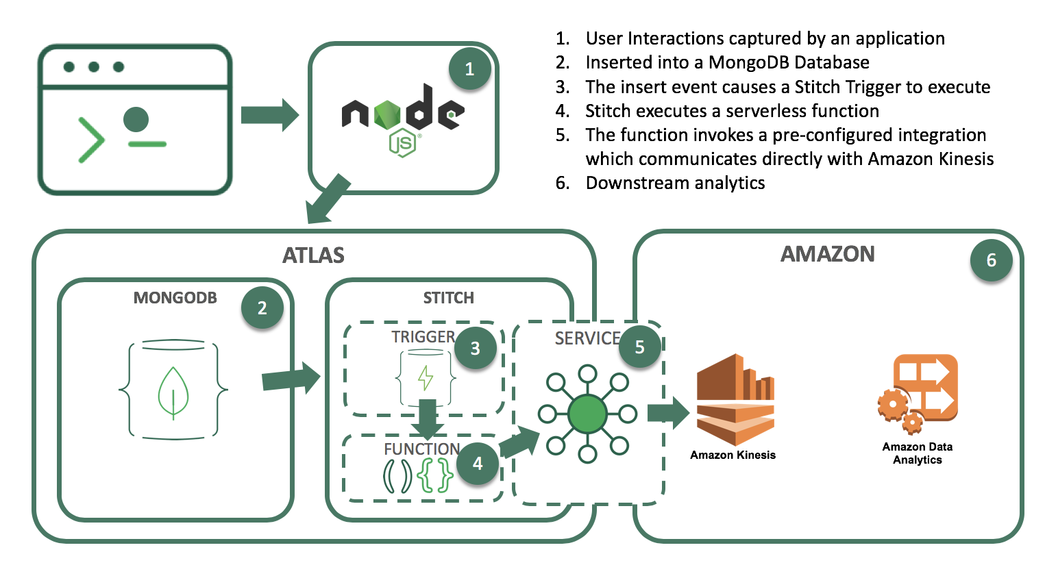
Let’s look at an example scenario in which a stream of data is being generated as a result of actions users take on a website. We’ll durably store the data and simultaneously feed a Kinesis process to do streaming analytics on something like cart abandonment, product recommendations, or even credit card fraud detection.

We’ll do this by setting up a Stitch Trigger. When relevant data updates are made in MongoDB, the trigger will use a Stitch Function to call out to AWS Kinesis, as you can see in this architecture diagram:

What you’ll need to follow along:

1. An Atlas instance
   If you don’t already have an application running on Atlas, you can follow our getting started with Atlas guide here. In this example, we’ll be using a database called streamdata, with a collection called clickdata where we’re writing data from our web-based e-commerce application.
2. An AWS account and a Kinesis stream
   In this example, we’ll use a Kinesis stream to send data downstream to additional applications such as Kinesis Analytics. This is the stream we want to feed our updates into.
3. A Stitch application
   If you don’t already have a Stitch application, log into Atlas, and click Stitch Apps from the navigation on the left, then click Create New Application.

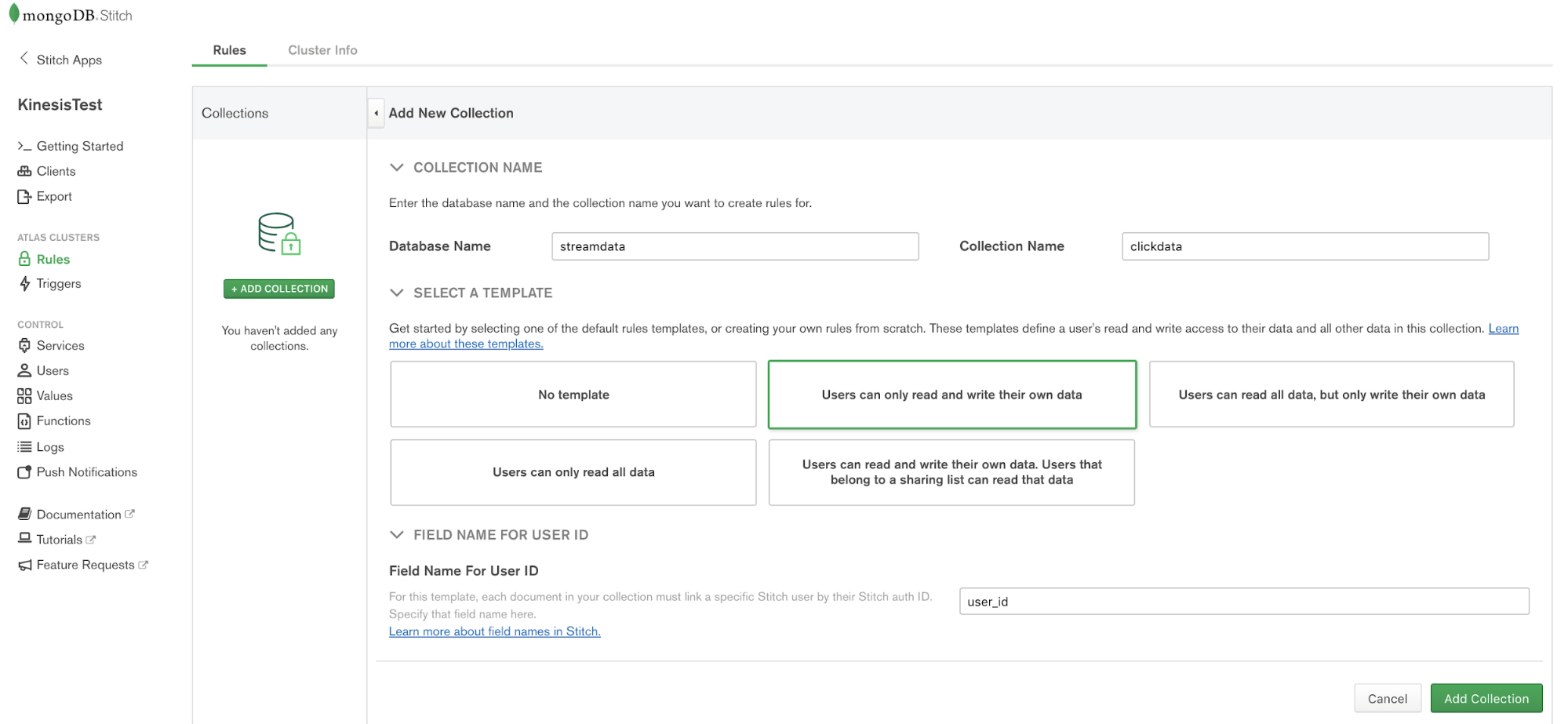
Create a Collection

The first step is to create a database and collection from the Stitch application console. Click Rules from the left navigation menu and click the Add Collection button. Type streamdata for the database and clickdata for the collection name. Select the template labeled Users can only read and write their own data and provide a field name where we’ll specify the user id.

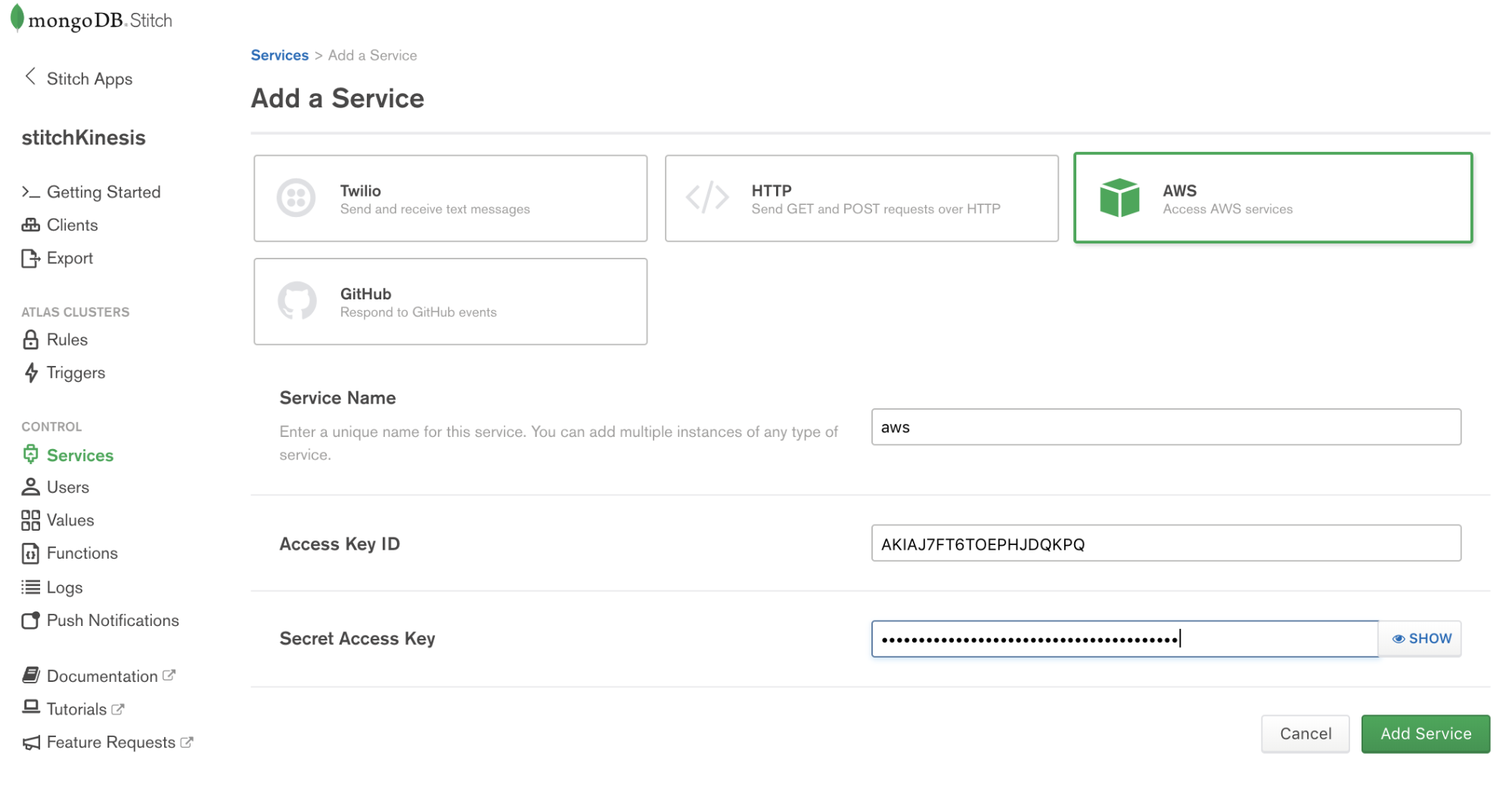
Configuring Stitch to talk to AWS

Stitch lets you configure Services to interact with external services such as AWS Kinesis. Choose Services from the navigation on the left, and click the Add a Service button, select the AWS service and set AWS Access Key ID, and Secret Access Key.

Services use Rules to specify what aspect of a service Stitch can use, and how. Add a rule which will enable that service to communicate with Kinesis by clicking the button labeled NEW RULE. Name the rule “kinesis” as we’ll be using this specific rule to enable communication with AWS Kinesis. In the section marked Action, select the API labeled Kinesis and select All Actions.

Write a function that uses the service to stream documents into Kinesis

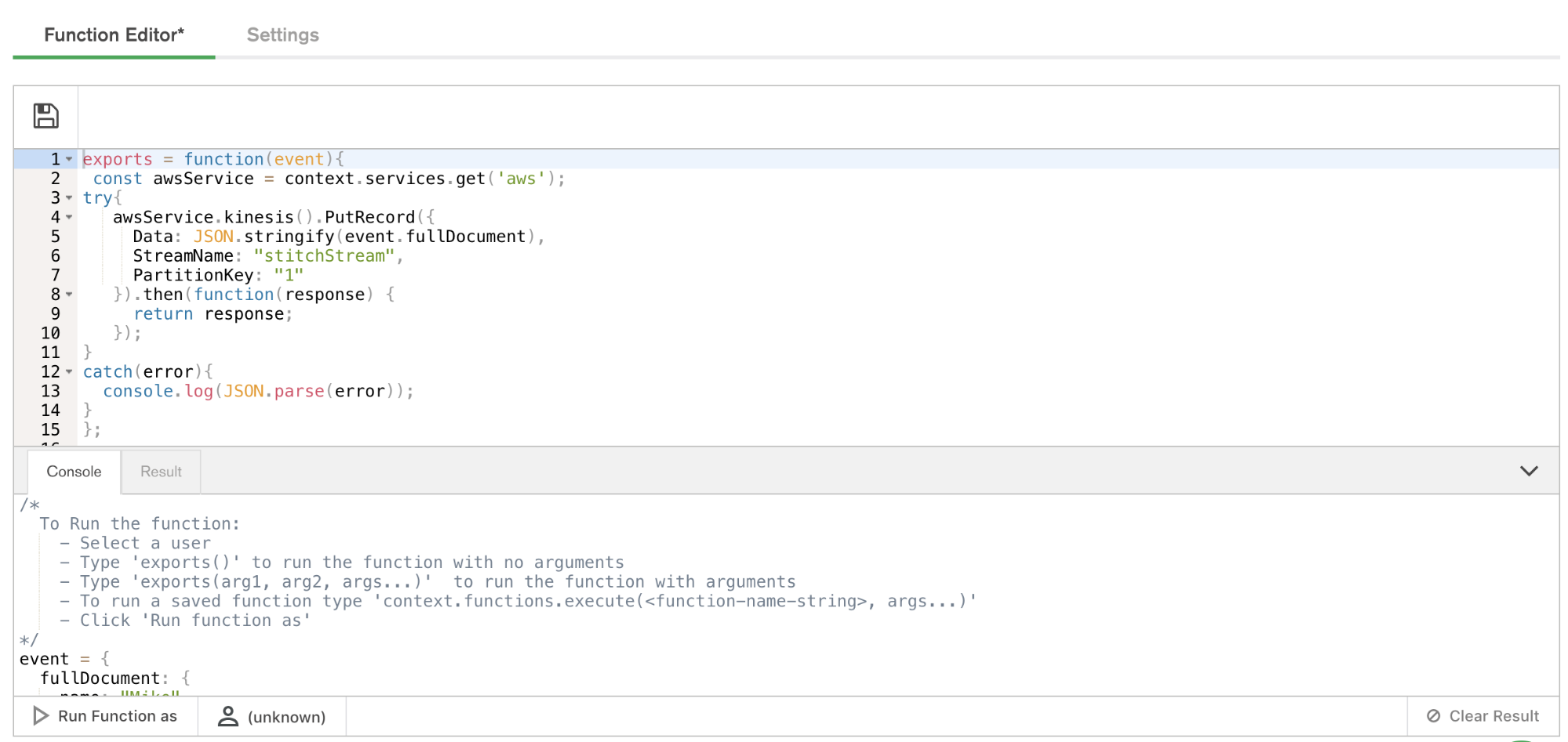
Now that we have a working AWS service, we can use it to put records into a Kinesis stream. The way we do that in Stitch is with Functions. Let’s set up a putKinesisRecord function.

Select Functions from the left-hand menu, and click Create New Function. Provide a name for the function and paste the following in the body of the function.

exports = function(event){
 const awsService = context.services.get('aws');
try{
   awsService.kinesis().PutRecord({
     Data: JSON.stringify(event.fullDocument),
     StreamName: "stitchStream",
     PartitionKey: "1"
      }).then(function(response) {
        return response;
      });
}
catch(error){
  console.log(JSON.parse(error));
}
};


Test out the function

Let’s make sure everything is working by calling that function manually. From the Function Editor, Click Console to view the interactive javascript console for Stitch.

Functions called from Triggers require an event. To test execution of our function, we’ll need to pass a dummy event to the function. Creating variables from the console in Stitch is simple. Simply set the value of the variable to a JSON document. For our simple example, use the following:

event = {
   "operationType": "replace",
   "fullDocument": {
       "color": "black",
       "inventory": {
           "$numberInt": "1"
       },
       "overview": "test document",
       "price": {
           "$numberDecimal": "123"
       },
       "type": "backpack"
   },
   "ns": {
       "db": "streamdata",
       "coll": "clickdata"
   }
}
exports(event);


Paste the above into the console and click the button labeled Run Function As. Select a user and the function will execute.

Ta-da!

Putting it together with Stitch Triggers

We’ve got our MongoDB collection living in Atlas, receiving events from our web app. We’ve got our Kinesis stream ready for data. We’ve got a Stitch Function that can put data into a Kinesis stream.

Configuring Stitch Triggers is so simple it’s almost anticlimactic. Click Triggers from the left navigation, name your trigger, provide the database and collection context, and select the database events Stitch will react to with execution of a function.

For the database and collection, use the names from step one. Now we’ll set the operations we want to watch with our trigger. (Some triggers might care about all of them – inserts, updates, deletes, and replacements – while others can be more efficient because they logically can only matter for some of those.) In our case, we’re going to watch for insert, update and replace operations.

Now we specify our putKinesisRecord function as the linked function, and we’re done.

As part of trigger execution, Stitch will forward details associated with the trigger event, including the full document involved in the event (i.e. the newly inserted, updated, or deleted document from the collection.) This is where we can evaluate some condition or attribute of the incoming document and decide whether or not to put the record onto a stream.

Test the trigger!

Amazon provides a dashboard which will enable you to view details associated with the data coming into your stream.

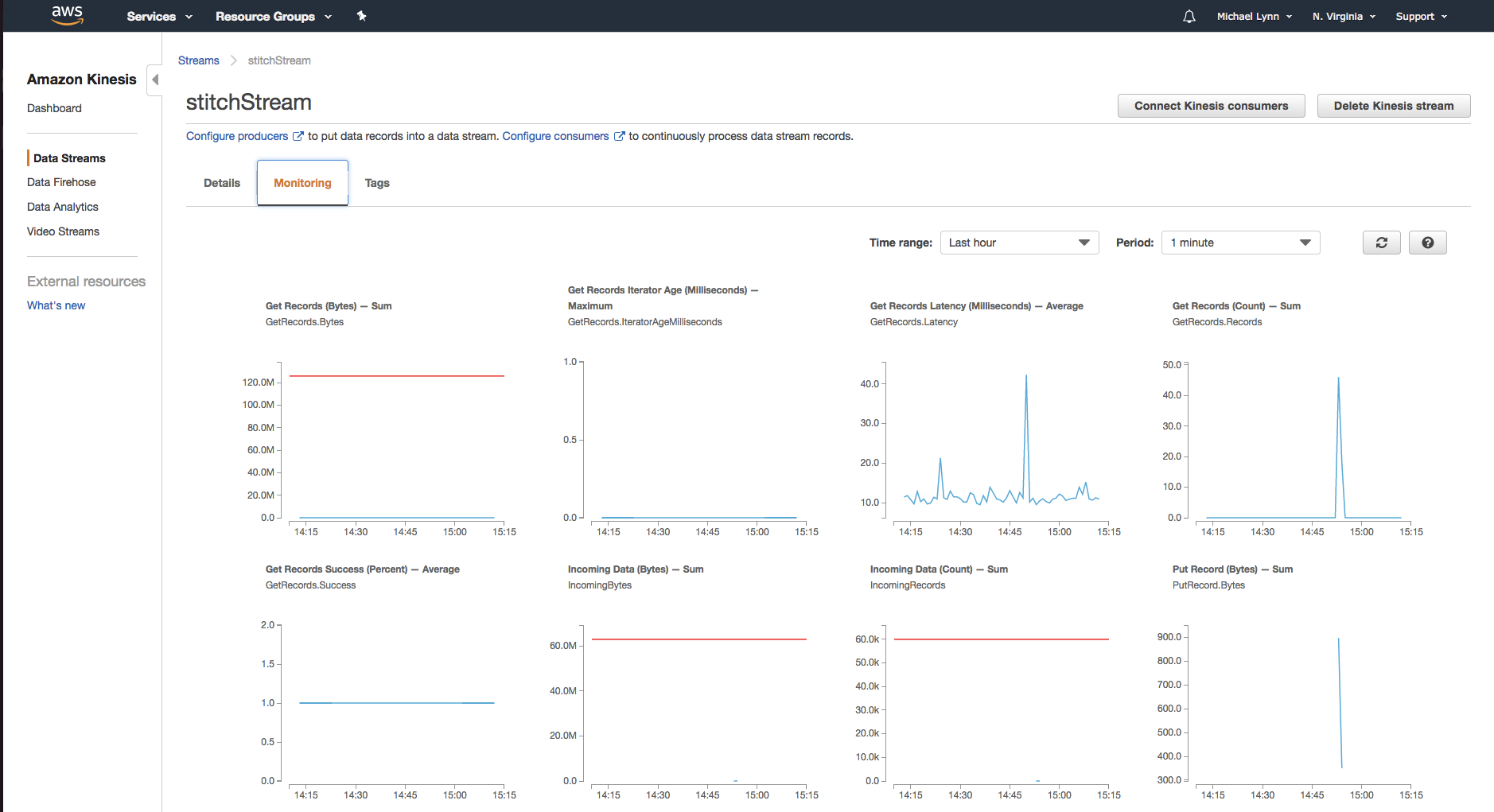
As you execute the function from within Stitch, you’ll begin to see the data entering the Kinesis stream.

Building some more functionality

So far our trigger is pretty basic – it watches a collection and when any updates or inserts happen, it feeds the entire document to our Kinesis stream. From here we can build out some more intelligent functionality. To wrap up this post, let’s look at what we can do with the data once it’s been durably stored in MongoDB and placed into a stream.

Once the record is in the Kinesis Stream you can configure additional services downstream to act on the data. A common use case incorporates Amazon Kinesis Data Analytics to perform analytics on the streaming data. Amazon Kinesis Data Analytics offers pre-configured templates to accomplish things like anomaly detection, simple alerts, aggregations, and more.

For example, our stream of data will contain orders resulting from purchases. These orders may originate from point-of-sale systems, as well as from our web-based e-commerce application. Kinesis Analytics can be leveraged to create applications that process the incoming stream of data. For our example, we could build a machine learning algorithm to detect anomalies in the data or create a product performance leaderboard from a sliding, or tumbling window of data from our stream.

Wrapping up

Now you can connect MongoDB to Kinesis. From here, you’re able to leverage any one of the many services offered from Amazon Web Services to build on your application. In our next article in the series, we’ll focus on getting the data back from Kinesis into MongoDB. In the meantime, let us know what you’re building with Atlas, Stitch, and Kinesis!

Resources

MongoDB Atlas

• Getting Started - Tutorial Playlist
• Signup for Free
• FAQ

MongoDB Stitch

• Getting Started Documentation
• MongoDB Stitch Tutorials
• MongoDB Stitch White Paper
• Webinar – 8th August 2018

Amazon Kinesis

• Getting Started
• Kinesis Data Streams
• Kinesis Data Analytics

Time-series data is increasingly at the heart of modern applications - think IoT, stock trading, clickstreams, social media, and more. With the move from batch to real time systems, the efficient capture and analysis of time-series data can enable organizations to better detect and respond to events ahead of their competitors, or to improve operational efficiency to reduce cost and risk. Working with time series data is often different from regular application data, and there are best practices you should observe. This blog series seeks to provide these best practices as you build out your time series application on MongoDB:

1. Introduce the concept of time-series data, and describe some of the challenges associated with this type of data
2. How to query, analyze and present time-series data
3. Provide discovery questions that will help you gather technical requirements needed for successfully delivering a time-series application.

What is time-series data?

While not all data is time-series in nature, a growing percentage of it can be classified as time-series – fueled by technologies that allow us to exploit streams of data in real time rather than in batches. In every industry and in every company there exists the need to query, analyze and report on time-series data. Consider a stock day trader constantly looking at feeds of stock prices over time and running algorithms to analyze trends in identify opportunities. They are looking at data over a time interval, e.g. hourly or daily ranges. A connected car company might obtain telemetry such as engine performance and energy consumption to improve component design, and monitor wear rates so they can schedule vehicle servicing before problems occur. They are also looking at data over a time interval.

Why is time-series data challenging?

Time-series data can include data that is captured at constant time intervals – like a device measurement per second – or at irregular time intervals like those generated from alerts and auditing event use cases. Time-series data is also often tagged with attributes like the device type and location of the event, and each device may provide a variable amount of additional metadata. Data model flexibility to meet diverse and rapidly changing data ingestion and storage requirements make it difficult for traditional relational (tabular) database systems with a rigid schema to effectively handle time-series data. Also, there is the issue of scalability. With a high frequency of readings generated by multiple sensors or events, time series applications can generate vast streams of data that need to be ingested and analyzed. So platforms that allow data to be scaled out and distributed across many nodes are much more suited to this type of use case than scale-up, monolithic tabular databases.

Time series data can come from different sources, with each generating different attributes that need to be stored and analyze. Each stage of the data lifecycle places different demands on a database – from ingestion through to consumption and archival.

• During data ingestion, the database is primarily performing write intensive operations, comprising mainly inserts with occasional updates. Consumers of data may want to be alerted in real time when an anomaly is detected in the data stream during ingestion, such as a value exceeding a certain threshold.
• As more data is ingested consumers may want to query it for specific insights, and to uncover trends. At this stage of the data lifecycle, the workload is read, rather than write heavy, but the database will still need to maintain high write rates as data is concurrently ingested and then queried.
• Consumers may want to query historical data and perform predictive analytics leveraging machine learning algorithms to anticipate future behavior or identify trends. This will impose additional read load on the database.
• In the end, depending on the application’s requirements, the data captured may have a shelf life and needs to be archived or deleted after a certain period of time.

As you can see working with time-series data is not just simply storing the data, but requires a wide range of data platform capabilities including handling simultaneous read and write demands, advanced querying capabilities, and archival to name a few.

Who is using MongoDB for time-series data?

MongoDB provides all the capabilities needed to meet the demands of a highly performing time-series applications. One company that took advantage of MongoDB’s time series capabilities is Quantitative Investment Manager Man AHL.

Man AHL’s Arctic application leverages MongoDB to store high frequency financial services market data (about 250M ticks per second). The hedge fund manager’s quantitative researchers (“quants”) use Arctic and MongoDB to research, construct and deploy new trading models in order to understand how markets behave. With MongoDB, Man AHL realized a 40x cost saving when compared to an existing proprietary database. In addition to cost savings, they were able to increase processing performance by 25x over the previous solution. Man AHL open sourced their Arctic project on GitHub.

Bosch Group is a multinational engineering conglomerate with nearly 300,000 employees and is the world’s largest automotive components manufacturer. IoT is a strategic initiative at Bosch, and so the company selected MongoDB as the data platform layer in its IoT suite. The suite powers IoT applications both within the Bosch group and in many of its customers in industrial internet applications, such as automotive, manufacturing, smart city, precision agriculture, and more. If you want to learn more about the key challenges presented by managing diverse, rapidly changing and high volume time series data sets generated by IoT platforms, download the Bosch and MongoDB whitepaper.

Siemens is a global company focusing on the areas of electrification, automation and digitalization. Siemens developed “Monet,” a platform backed by MongoDB that provides advanced energy management services. Monet uses MongoDB for real time raw data storage, querying and analytics.

Focus on application requirements

When working with time-series data it is imperative that you invest enough time to understand how data is going to be created, queried, and expired. With this information you can optimize your schema design and deployment architecture to best meet the application’s requirements.

You should not agree to performance metrics or SLAs without capturing the application’s requirements.

As you begin your time-series project with MongoDB you should get answers to the following questions:

Write workload

• What will the ingestion rate be? How many inserts and updates per second?
As the rate of inserts increases, your design may benefit from horizontal scaling via MongoDB auto-sharding, allowing you to partition and scale your data across many nodes
• How many simultaneous client connections will there be?
While a single MongoDB node can handle many simultaneous connections from tens of thousands of IoT devices, you need to consider scaling those out with sharding to meet the expected client load.
• Do you need to store all raw data points or can data be pre-aggregated? If pre-aggregated, what summary level of granularity or interval is acceptable to store? Per minute? Every 15 minutes?
MongoDB can store all your raw data if you application requirements justify this. However, keep in mind that reducing the data size via pre-aggregation will yield lower dataset and index storage and an increase in query performance.
• What is the size of data stored in each event?
MongoDB has an individual document size limit of 16 MB. If your application requires storing larger data within a single document, such as binary files you may want to leverage MongoDB GridFS. Ideally when storing high volume time-series data it is a best practice to keep the document size small around 1 disk block size.

Read workload:

• How many read queries per second?
A higher read query load may benefit from additional indexes or horizontal scaling via MongoDB auto-sharding.
As with write volumes, reads can be scaled with auto-sharding. You can also distribute read load across secondary replicas in your replica set.
• Will clients be geographically dispersed or located in the same region?
You can reduce network read latency by deploying read-only secondary replicas that are geographically closer to the consumers of the data.
• What are the common data access patterns you need to support? For example, will you retrieve data by a single value such as time, or do you need more complex queries where you look for data by a combination of attributes, such as event class, by region, by time?
Query performance is optimal when proper indexes are created. Knowing how data is queried and defining the proper indexes is critical to database performance. Also, being able to modify indexing strategies in real time, without disruption to the system, is an important attribute of a time-series platform.
• What analytical libraries or tools will your consumers use?
If your data consumers are using tools like Hadoop or Spark, MongoDB has a MongoDB Spark Connector that integrates with these technologies. MongoDB also has drivers for Python, R, Matlab and other platforms used for analytics and data science.
• Does your organization use BI visualization tools to create reports or analyze the data?
MongoDB integrates with most of the major BI reporting tools including Tableau, QlikView, Microstrategy, TIBCO, and others via the MongoDB BI Connector. MongoDB also has a native BI reporting tool called MongoDB Charts, which provides the fastest way to visualize your data in MongoDB without needing any third-party products.

• What is the data retention policy? Can data be deleted or archived? If so, at what age?
• If archived, for how long and how accessible should the archive be? Does archive data need to be live or can it be restored from a backup?
There are various strategies to remove and archive data in MongoDB. Some of these strategies include using TTL indexes, Queryable Backups, zoned sharding (allowing you to create a tiered storage pattern), or simply creating an architecture where you just drop the collection of data when no longer needed.

Security:

• What users and roles need to be defined, and what is the least privileged permission needed for each of these entities?
• What are the encryption requirements? Do you need to support both in-flight (network) and at-rest (storage) encryption of time series data?
• Do all activities against the data need to be captured in an audit log?
• Does the application need to conform with GDPR, HIPAA, PCI, or any other regulatory framework?
The regulatory framework may require enabling encryption, auditing, and other security measures. MongoDB supports the security configurations necessary for these compliances, including encryption at rest and in flight, auditing, and granular role-based access control controls.

While not an exhaustive list of all possible things to consider, it will help get you thinking about the application requirements and their impact on the design of the MongoDB schema and database configuration. In the next blog post, "Part 2: Schema design for time-series data in MongoDB” we will explore a variety of ways to architect a schema for different sets of requirements, and their corresponding effects on the application’s performance and scale. In part 3, "Time Series Data and MongoDB: Part 3 – Querying, Analyzing, and Presenting Time-Series Data", we will show how to query, analyze and present time-series data.

Welcome to PyMongo Monday. This is the first in a series of regular blog posts that will introduce developers to programming MongoDB using the Python programming language. It’s called PyMongo Monday because PyMongo is the name of the client library (in MongoDB speak we refer to it as a "driver") we use to interact with the MongoDB Server. Monday because we aim to release each new episode on Monday.

To get started we need to install the toolchain used by a typical MongoDB Python developer.

Installing m

First up is m. Hard to find online unless your search for "MongoDB m", m is a tool to manage and use multiple installations of the MongoDB Server in parallel. It is an invaluable tool if you want to try out the latest and greatest beta version but still continue mainline development on our current stable release.

The easiest way to install m is with npm the Node.js package manager (which it turns out is not just for Node.js).

$ sudo npm install -g m
Password:******
/usr/local/bin/m -> /usr/local/lib/node_modules/m/bin/m
+ m@1.4.1
updated 1 package in 2.361s
$

If you can’t or don’t want to use npm you can download and install directly from the github repo. See the README there for details.

For today we will use m to install the current stable production version (4.0.2 at the time of writing).

We run the stable command to achieve this.

$ m stable
MongoDB version 4.0.2 is not installed.
Installation may take a while. Would you like to proceed? [y/n] y
... installing binary

######################################################################## 100.0%
/Users/jdrumgoole
... removing source
... installation complete
$

If you need to use the path directly in another program you can get that with m bin.

$ m bin 4.0.0
/usr/local/m/versions/4.0.1/bin
$

To run the corresponding binary do m use stable

$ m use stable
2018-08-28T11:41:48.157+0100 I CONTROL  [main] Automatically disabling TLS 1.0, to force-enable TLS 1.0 specify --sslDisabledProtocols 'none'
2018-08-28T11:41:48.171+0100 I CONTROL  [initandlisten] MongoDB starting : pid=38524 port=27017 dbpath=/data/db 64-bit host=JD10Gen.local
2018-08-28T11:41:48.171+0100 I CONTROL  [initandlisten] db version v4.0.2
2018-08-28T11:41:48.171+0100 I CONTROL  [initandlisten] git version: fc1573ba18aee42f97a3bb13b67af7d837826b47
&lt other server output &gt
...
2018-06-13T15:52:43.648+0100 I NETWORK  [initandlisten] waiting for connections on port 27017

Now that we have a server running we can confirm that it works by connecting via the mongo shell.

$ mongo
MongoDB shell version v4.0.0
connecting to: mongodb://127.0.0.1:27017
MongoDB server version: 4.0.0
Server has startup warnings:
2018-07-06T10:56:50.973+0100 I CONTROL  [initandlisten]
2018-07-06T10:56:50.973+0100 I CONTROL  [initandlisten] ** WARNING: Access control is not enabled for the database.
2018-07-06T10:56:50.973+0100 I CONTROL  [initandlisten] **          Read and write access to data and configuration is unrestricted.
2018-07-06T10:56:50.973+0100 I CONTROL  [initandlisten] ** WARNING: You are running this process as the root user, which is not recommended.
2018-07-06T10:56:50.973+0100 I CONTROL  [initandlisten]
2018-07-06T10:56:50.973+0100 I CONTROL  [initandlisten] ** WARNING: This server is bound to localhost.
2018-07-06T10:56:50.973+0100 I CONTROL  [initandlisten] **          Remote systems will be unable to connect to this server.
2018-07-06T10:56:50.973+0100 I CONTROL  [initandlisten] **          Start the server with --bind_ip &lt address&gt to specify which IP
2018-07-06T10:56:50.973+0100 I CONTROL  [initandlisten] **          addresses it should serve responses from, or with --bind_ip_all to
2018-07-06T10:56:50.973+0100 I CONTROL  [initandlisten] **          bind to all interfaces. If this behavior is desired, start the
2018-07-06T10:56:50.973+0100 I CONTROL  [initandlisten] **          server with --bind_ip 127.0.0.1 to disable this warning.
2018-07-06T10:56:50.973+0100 I CONTROL  [initandlisten]

---
Enable MongoDB's free cloud-based monitoring service to collect and display
metrics about your deployment (disk utilization, CPU, operation statistics,
etc).

The monitoring data will be available on a MongoDB website with a unique
URL created for you. Anyone you share the URL with will also be able to
view this page. MongoDB may use this information to make product
improvements and to suggest MongoDB products and deployment options to you.

To enable free monitoring, run the following command:
db.enableFreeMonitoring()
---

>

These warnings are standard. They flag that this database has no access controls setup by default and, that it is only listening to connections coming from the machine it is running on (localhost). We will learn how to setup access control and listen on a broader range of ports in later episodes.

Installing the PyMongo Driver

But this series is not about the MongoDB Shell, which uses JavaScript as its coin of the realm, it’s about Python. How do we connect to the database with Python?

First we need to install the MongoDB Python Driver, PyMongo. In MongoDB parlance a driver is a language-specific client library that allows developers to interact with the server in the idiom of their own programming language.

For Python that means installing the driver with pip. In node.js the driver is installed using npm and in Java you can use maven.

$ pip3 install pymongo
Collecting pymongo
  Downloading https://files.pythonhosted.org/packages/a1/e0/51df08036e04c1ddc985a2dceb008f2f21fc1d6de711bb6cee85785c1d78/pymongo-3.7.1-cp27-cp27m-macosx_10_13_intel.whl (333kB)
    100% |████████████████████████████████| 337kB 4.1MB/s
Installing collected packages: pymongo
Successfully installed pymongo-3.7.1
$

We recommend you use a virtual environment to isolate your PyMongo Monday code. This is not required but is very convenient for isolating different development streams.

Now we can connect to the database:

$ python
Python 3.6.5 (v3.6.5:f59c0932b4, Mar 28 2018, 03:03:55)
[GCC 4.2.1 (Apple Inc. build 5666) (dot 3)] on darwin
Type "help", "copyright", "credits" or "license" for more information.
>>> import pymongo                                                  (1)
>>> client = pymongo.MongoClient(host="mongodb://localhost:8000")   (2)
>>> result = client.admin.command("isMaster")                       (3)
>>> import pprint
>>> pprint.pprint(result)
{'ismaster': True,
 'localTime': datetime.datetime(2018, 6, 13, 21, 55, 2, 272000),
 'logicalSessionTimeoutMinutes': 30,
 'maxBsonObjectSize': 16777216,
 'maxMessageSizeBytes': 48000000,
 'maxWireVersion': 6,
 'maxWriteBatchSize': 100000,
 'minWireVersion': 0,
 'ok': 1.0,
 'readOnly': False}
>>>

First we import the PyMongo library (1). Then we create a local client object (2) that holds the connection pool and other status for this server. We generally don’t want more than one MongoClient object per program as it provides its own connection pool.

Now we are ready to issue a command to the server. In this case it's the standard MongoDB server information command which is called rather anachronistically isMaster (3). This is a hangover from the very early versions of MongoDB. It appears in pre 1.0 versions of MongoDB (which is over ten years old at this stage). The isMaster command returns a dict which details a bunch of server information. In order to format this in a more readable way we import the pprint library.

Conclusion

That’s the end of episode one. We have installed MongoDB, installed the Python client library (aka driver), started a mongod server and established a connection between the client and server.

Next week we will introduce CRUD operations on MongoDB, starting with Create.

For direct feedback please pose your questions on twitter/jdrumgoole. That way everyone can see the answers.

The best way to try out MongoDB is via MongoDB Atlas our fully managed Database as a Service available on AWS, Google Cloud Platform (CGP) and Azure.

In the previous blog post, “Time Series Data and MongoDB: Part 1 – An Introduction,” we introduced the concept of time-series data followed by some discovery questions you can use to help gather requirements for your time-series application. Answers to these questions help guide the schema and MongoDB database configuration needed to support a high-volume production application deployment. In this blog post we will focus on how two different schema designs can impact memory and disk utilization under read, write, update, and delete operations.

In the end of the analysis you may find that the best schema design for your application may be leveraging a combination of schema designs. By following the recommendations we lay out below, you will have a good starting point to develop the optimal schema design for your app, and appropriately size your environment.

Designing a time-series schema

Let’s start by saying that there is no one canonical schema design that fits all application scenarios. There will always be trade-offs to consider regardless of the schema you develop. Ideally you want the best balance of memory and disk utilization to yield the best read and write performance that satisfy your application requirements, and that enables you to support both data ingest and analysis of time-series data streams.

In this blog post we will look at various schema design configurations. First, storing one document per data sample, and then bucketing the data using one document per time-series time range and one document per fixed size. Storing more than one data sample per document is known as bucketing. This will be implemented at the application level and requires nothing to be configured specifically in MongoDB. With MongoDB’s flexible data model you can optimally bucket your data to yield the best performance and granularity for your application’s requirements.

This flexibility also allows your data model to adapt to new requirements over time – such as capturing data from new hardware sensors that were not part of the original application design. These new sensors provide different metadata and properties than the sensors you used in the original design. WIth all this flexibility you may think that MongoDB databases are the wild west, where anything goes and you can quickly end up with a database full of disorganized data. MongoDB provides as much control as you need via schema validation that allows you full control to enforce things like the presence of mandatory fields and range of acceptable values, to name a few.

To help illustrate how schema design and bucketing affects performance, consider the scenario where we want to store and analyze historical stock price data. Our sample stock price generator application creates sample data every second for a given number of stocks that it tracks. One second is the smallest time interval of data collected for each stock ticker in this example. If you would like to generate sample data in your own environment, the StockGen tool is available on GitHub. It is important to note that although the sample data in this document uses stock ticks as an example, you can apply these same design concepts to any time-series scenario like temperature and humidity readings from IoT sensors.

The StockGen tool used to generate sample data will generate the same data and store it in two different collections: StockDocPerSecond and StockDocPerMinute that each contain the following schemas:

Scenario 1: One document per data point

{
  "_id" : ObjectId("5b4690e047f49a04be523cbd"),
"p" : 56.56,
  "symbol" : "MDB",
  "d" : ISODate("2018-06-30T00:00:01Z")
},
{
  "_id" : ObjectId("5b4690e047f49a04be523cbe"),
"p" : 56.58,
  "symbol" : "MDB",
  "d" : ISODate("2018-06-30T00:00:02Z")
}
,...


Scenario 2: Time-based bucketing of one document per minute

{
"_id" : ObjectId("5b5279d1e303d394db6ea0f8"), 
"p" : {
"0" : 56.56,
"1" : 56.56,
"2" : 56.58,
…
"59" : 57.02
},
"symbol" : "MDB",
"d" : ISODate("2018-06-30T00:00:00Z")
},
{
"_id" : ObjectId("5b5279d1e303d394db6ea134"), 
"p" : {
 "0" : 69.47,
 "1" : 69.47,
 "2" : 68.46,
...
 "59" : 69.45
},
"symbol" : "TSLA",
"d" : ISODate("2018-06-30T00:01:00Z")
},...


Note that the field “p” contains a subdocument with the values for each second of the minute.

Schema design comparisons

Let’s compare and contrast the database metrics of storage size and memory impact based off of 4 weeks of data generated by the StockGen tool. Measuring these metrics is useful when assessing database performance.

Effects on Data Storage

In our application the smallest level of time granularity is a second. Storing one document per second as described in Scenario 1 is the most comfortable model concept for those coming from a relational database background. That is because we are using one document per data point, which is similar to a row per data point in a tabular schema. This design will produce the largest number of documents and collection size per unit of time as seen in Figures 3 and 4.

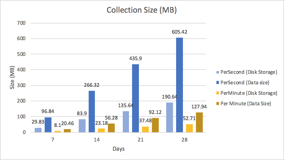
Figure 4 shows two sizes per collection. The first value in the series is the size of the collection that is stored on disk, while the second value is the size of the data in the database. These numbers are different because MongoDB’s WiredTiger storage engine supports compression of data at rest. Logically the PerSecond collection is 605MB, but on disk it is consuming around 190 MB of storage space.

Effects on memory utilization

A large number of documents will not only increase data storage consumption but increase index size as well. An index was created on each collection and covered the symbol and date fields. Unlike some key-value databases that position themselves as time-series databases, MongoDB provides secondary indexes giving you flexible access to your data and allowing you to optimize query performance of your application.

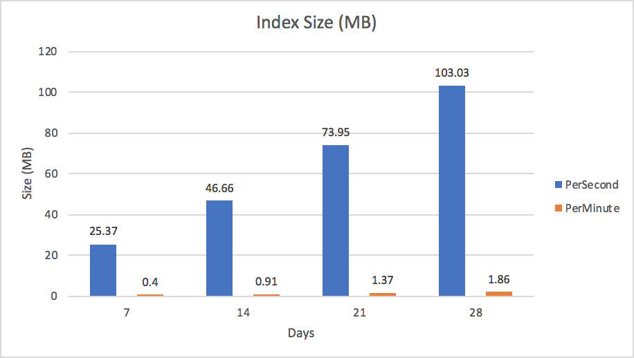
The size of the index defined in each of the two collections IS seen in Figure 5. Optimal performance of MongoDB happens when indexes and most recently used documents fit into the memory allocated by the WiredTiger cache (we call this the “working set”). In our example we generated data for just 5 stocks over the course of 4 weeks. Given this small test case our data already generated an index that is 103MB in size for the PerSecond scenario. Keep in mind that there are some optimizations such as index prefix compression that help reduce the memory footprint of an index. However, even with these kind of optimizations proper schema design is important to prevent runaway index sizes. Given the trajectory of growth, any changes to the application requirements, like tracking more than just 5 stocks or more than 4 weeks of prices in our sample scenario, will put much more pressure on memory and eventually require indexes to page out to disk. When this happens your performance will be degraded. To mitigate this situation, consider scaling horizontally.

Scale horizontally

As your data grows in size you may end up scaling horizontally when you reach the limits of the physical limits of the server hosting the primary mongod in your MongoDB replica set.

By horizontally scaling via MongoDB Sharding, performance can be improved since the indexes and data will be spread over multiple MongoDB nodes. Queries are no longer directed at a specific primary node. Rather they are processed by an intermediate service called a query router (mongos), which sends the query to the specific nodes that contain the data that satisfy the query. Note that this is completely transparent to the application – MongoDB handles all of the routing for you

Scenario 3: Size-based bucketing

The key takeaway when comparing the previous scenarios is that bucketing data has significant advantages. Time-based bucketing as described in scenario 2 buckets an entire minute's worth of data into a single document. In time-based applications such as IoT, sensor data may be generated at irregular intervals and some sensors may provide more data than others. In these scenarios, time-based bucketing may not be the optimal approach to schema design. An alternative strategy is size-based bucketing. With size-based bucketing we design our schema around one document per a certain number of emitted sensor events, or for the entire day, whichever comes first.

To see size-based bucketing in action, consider the scenario where you are storing sensor data and limiting the bucket size to 200 events per document, or a single day (whichever comes first). Note: The 200 limit is an arbitrary number and can be changed as needed, without application changes or schema migrations.

{
  _id: ObjectId(),
 deviceid: 1234,
 sensorid: 3,
 nsamples: 5,
  day: ISODate("2018-08-29"),
 first:1535530412,
 last: 1535530432,
 samples : [
   { val: 50, time: 1535530412},
   { val: 55, time : 1535530415},
   { val: 56, time: 1535530420},
   { val: 55, time : 1535530430},
   { val: 56, time: 1535530432}
   ]
}


An example size-based bucket is shown in figure 6. In this design, trying to limit inserts per document to an arbitrary number or a specific time period may seem difficult; however, it is easy to do using an upsert, as shown in the following code example:

sample = {val: 59, time: 1535530450}
day = ISODate("2018-08-29")
db.iot.updateOne({deviceid: 1234, sensorid: 3, nsamples: {$lt: 200}, day: day},
                 {$push: {samples: sample},
                  $min: {first: sample.time},
                  $max: {last: sample.time},
                  $inc: {nsamples: 1}, {upsert: true} )


As new sensor data comes in it is simply appended to the document until the number of samples hit 200, then a new document is created because of our upsert:true clause.

The optimal index in this scenario would be on {deviceid:1,sensorid:1,day:1,nsamples:1}. When we are updating data, the day is an exact match, and this is super efficient. When querying we can specify a date, or a date range on a single field which is also efficient as well as filtering by first and last using UNIX timestamps. Note that we are using integer values for times. These are really times stored as a UNIX timestamp and only take 32 bits of storage versus an ISODate which takes 64 bits. While not a significant query performance difference over ISODate, storing as UNIX timestamp may be significant if you plan on ending up with terabytes of ingested data and you do not need to store a granularity less than a second.

Bucketing data in a fixed size will yield very similar database storage and index improvements as seen when bucketing per time in scenario 2. It is one of the most efficient ways to store sparse IoT data in MongoDB.

What to do with old data

Should we store all data in perpetuity? Is data older than a certain time useful to your organization? How accessible should older data be? Can it be simply restored from a backup when you need it, or does it need to be online and accessible to users in real time as an active archive for historical analysis? As we covered in part 1 of this blog series, these are some of the questions that should be asked prior to going live.

There are multiple approaches to handling old data and depending on your specific requirements some may be more applicable than others. Choose the one that best fits your requirements.

Pre-aggregation

Does your application really need a single data point for every event generated years ago? In most cases the resource cost of keeping this granularity of data around outweighs the benefit of being able to query down to this level at any time. In most cases data can be pre-aggregated and stored for fast querying. In our stock example, we may want to only store the closing price for each day as a value. In most architectures, pre-aggregated values are stored in a separate collection since typically queries for historical data are different than real-time queries. Usually with historical data, queries are looking for trends over time versus individual real-time events. By storing this data in different collections you can increase performance by creating more efficient indexes as opposed to creating more indexes on top of real-time data.

Offline archival strategies

When data is archived, what is the SLA associated with retrieval of the data? Is restoring a backup of the data acceptable or does the data need to be online and ready to be queried at any given time? Answers to these questions will help drive your archive design. If you do not need real-time access to archival data you may want to consider backing up the data and removing it from the live database. Production databases can be backed up using MongoDB Ops Manager or if using the MongoDB Atlas service you can use a fully managed backup solution.

Removing documents using remove statement

Once data is copied to an archival repository via a database backup or an ETL process, data can be removed from a MongoDB collection via the remove statement as follows:

 db.StockDocPerSecond.remove ( { "d" : { $lt: ISODate( "2018-03-01" ) } } )

In this example all documents that have a date before March 1st, 2018 defined on the “d” field will be removed from the StockDocPerSecond collection.

You may need to set up an automation script to run every so often to clean out these records. Alternatively, you can avoid creating automation scripts in this scenario by defining a time to live (TTL) index.

Removing documents using a TTL Index

A TTL index is similar to a regular index except you define a time interval to automatically remove documents from a collection. In the case of our example, we could create a TTL index that automatically deletes data that is older than 1 week.

db.StockDocPerSecond.createIndex( { "d": 1 }, { expireAfterSeconds: 604800 } )

Although TTL indexes are convenient, keep in mind that the check happens every minute or so and the interval cannot be configured. If you need more control so that deletions won’t happen during specific times of the day you may want to schedule a batch job that performs the deletion in lieu of using a TTL index.

Removing documents by dropping the collection

It is important to note that using the remove command or TTL indexes will cause high disk I/O. On a database that may be under high load already this may not be desirable. The most efficient and fastest way to remove records from the live database is to drop the collection. If you can design your application such that each collection represents a block of time, \ when you need to archive or remove data all you need to do is drop the collection. This may require some smarts within your application code to know which collections should be queried, but the benefit may outweigh this change. When you issue a remove, MongoDB also has to remove data from all affected indexes as well and this could take a while depending on the size of data and indexes.

Online archival strategies

If archival data still needs to be accessed in real time, consider how frequently these queries occur and if storing only pre-aggregated results can be sufficient.

Sharding archival data

One strategy for archiving data and keeping the data accessible real-time is by using zoned sharding to partition the data. Sharding not only helps with horizontally scaling the data out across multiple nodes, but you can tag shard ranges so partitions of data are pinned to specific shards. A cost saving measure could be to have the archival data live on shards running lower cost disks and periodically adjusting the time ranges defined in the shards themselves. These ranges would cause the balancer to automatically move the data between these storage layers, providing you with tiered, multi-temperature storage. Review our tutorial for creating tiered storage patterns with zoned sharding for more information.

Accessing archived data via queryable backups

If your archive data is not accessed that frequently and the query performance does not need to meet any strict latency SLAs, consider backing the data up and using the Queryable Backups feature of MongoDB Atlas or MongoDB OpsManager. Queryable Backups allow you to connect to your backup and issue read-only commands to the backup itself, without having to first restore the backup.

Querying data from the data lake

MongoDB is an inexpensive solution not only for long term archival but for your data lake as well. Companies who have made investments in technologies like Apache Spark can leverage the MongoDB Spark Connector. This connector materializes MongoDB data as DataFrames and Datasets for use with Spark and machine learning, graph, streaming, and SQL APIs.

Key Takeaways

Once an application is live in production and is multiple terabytes in size, any major change can be very expensive from a resource standpoint. Consider the scenario where you have 6 TB of IoT sensor data and are accumulating new data at a rate of 50,000 inserts per second. Performance of reads is starting to become an issue and you realize that you have not properly scaled out the database. Unless you are willing to take application downtime, a change of schema in this configuration – e.g., moving from raw data storage to bucketed storage – may require building out shims, temporary staging areas and all sorts of transient solutions to move the application to the new schema. The moral of the story is to plan for growth and properly design the best time-series schema that fits your application’s SLAs and requirements.

This article analyzed two different schema designs for storing time-series data from stock prices. Is the schema that won in the end for this stock price database the one that will be the best in your scenario? Maybe. Due to the nature of time-series data and the typical rapid ingestion of data the answer may in fact be leveraging a combination of collections that target a read or write heavy use case. The good news is that with MongoDB’s flexible schema, it is easy to make changes. In fact you can run two different versions of the app writing two different schemas to the same collection. However, don’t wait until your query performance starts suffering to figure out an optimal design as migrating TBs of existing documents into a new schema can take time and resources, and delay future releases of your application. You should undertake real world testing before commiting on a final design. Quoting a famous proverb, “Measure twice and cut once.”

In the next blog post, “Querying, Analyzing, and Presenting Time-Series Data with MongoDB,” we will look at how to effectively get value from the time-series data stored in MongoDB.

Key Tips:

• The MMAPV1 storage engine is deprecated, so use the default WiredTiger storage engine. Note that if you read older schema design best practices from a few years ago, they were often built on the older MMAPV1 technology.
• Understand what the data access requirements are from your time-series application.
• Schema design impacts resources. “Measure twice and cut once” with respect to schema design and indexes.
• Test schema patterns with real data and a real application if possible.
• Bucketing data reduces index size and thus massively reduces hardware requirements.
• Time-series applications traditionally capture very large amounts of data, so only create indexes where they will be useful to the app’s query patterns.
• Consider more than one collection: one focused on write heavy inserts and recent data queries and another collection with bucketed data focused on historical queries on pre-aggregated data.
• When the size of your indexes exceeds the amount of memory on the server hosting MongoDB, consider horizontally scaling out to spread the index and load over multiple servers.
• Determine at what point data expires, and what action to take, such as archival or deletion.

Last time we showed you how to setup up your environment.

In the next few episodes we will take you through the standard CRUD operators that every database is expected to support. In this episode we will focus on the Create in CRUD.

Create

Lets look at how we insert JSON documents into MongoDB.

First lets start a local single instance of mongod using m.

$ m use stable
2018-08-28T14:58:06.674+0100 I CONTROL [main] Automatically disabling TLS 1.0, to force-enable TLS 1.0 specify --sslDisabledProtocols 'none'
2018-08-28T14:58:06.689+0100 I CONTROL [initandlisten] MongoDB starting : pid=43658 port=27017 dbpath=/data/db 64-bit host=JD10Gen.local
2018-08-28T14:58:06.689+0100 I CONTROL [initandlisten] db version v4.0.2
2018-08-28T14:58:06.689+0100 I CONTROL [initandlisten] git version: fc1573ba18aee42f97a3bb13b67af7d837826b47
2018-08-28T14:58:06.689+0100 I CONTROL [initandlisten] allocator: syste

etc...

The mongod starts listening on port 27017 by default. As every MongoDB driver defaults to connecting on localhost:27017 we won't need to specify a connection string explicitly in these early examples.

Now, we want to work with the Python driver. These examples are using Python 3.6.5 but everything should work with versions as old as Python 2.7 without problems.

Unlike SQL databases, databases and collections in MongoDB only have to be named to be created. As we will see later this is a lazy creation process, and the database and corresponding collection are actually only created when a document is inserted.

$ python
Python 3.6.5 (v3.6.5:f59c0932b4, Mar 28 2018, 03:03:55)
[GCC 4.2.1 (Apple Inc. build 5666) (dot 3)] on darwin
Type "help", "copyright", "credits" or "license" for more information.
>>>
>>> import pymongo
>>> client = pymongo.MongoClient()
>>> database = client[ "ep002" ]
>>> people_collection = database[ "people_collection" ]
>>> result=people_collection.insert_one({"name" : "Joe Drumgoole"})
>>> result.inserted_id
ObjectId('5b7d297cc718bc133212aa94')
>>> result.acknowledged
True
>>> people_collection.find_one()
{'_id': ObjectId('5b62e6f8c3b498fbfdc1c20c'), 'name': 'Joe Drumgoole'}
True
>>>

First we import the pymongo library (line 6). Then we create the local client proxy object, client = pymongo.MongoClient() (line 7) . The client object manages a connection pool to the server and can be used to set many operational parameters related to server connections.

We can leave the parameter list to the MongoClient call blank. Remember, the server by default listens on port 27017 and the client by default attempts to connect to localhost:27017.

Once we have a client object, we can now create a database, ep002 (line 8) and a collection, people_collection (line 9). Note that we do not need an explicit DDL statement.

Using Compass to examine the database server

A database is effectively a container for collections. A collection provides a container for documents. Neither the database nor the collection will be created on the server until you actually insert a document. If you check the server by connecting MongoDB Compass you will see that there are no databases or collections on this server before the insert_one call.

These commands are lazily evaluated. So, until we actually insert a document into the collection, nothing happens on the server.

Once we insert a document:

>>>> result=database.people_collection.insert_one({"name" : "Joe Drumgoole"})
>>> result.inserted_id
ObjectId('5b7d297cc718bc133212aa94')
>>> result.acknowledged
True
>>> people_collection.find_one()
{'_id': ObjectId('5b62e6f8c3b498fbfdc1c20c'), 'name': 'Joe Drumgoole'}
True
>>>

We will see that the database, the collection, and the document are created.

And we can see the document in the database.

_id Field

Every object that is inserted into a MongoDB database gets an automatically generated _id field. This field is guaranteed to be unique for every document inserted into the collection. This unique property is enforced as the _id field is automatically indexed and the index is unique.

The value of the _id field is defined as follows:

The _id field is generated on the client and you can see the PyMongo generation code in the objectid.py file. Just search for the def _generate string. All MongoDB drivers generate _id fields on the client side. The _id field allows us to insert the same JSON object many times and allow each one to be uniquely identified. The _id field even gives a temporal ordering and you can get this from an ObjectID via the generation_time method.

>>> from bson import ObjectId
>>> x=ObjectId('5b7d297cc718bc133212aa94')
>>> x.generation_time
datetime.datetime(2018, 8, 22, 9, 14, 36, tzinfo=)
>>> <b>print(x.generation_time)</b>
2018-08-22 09:14:36+00:00
>>>

Wrap Up

That is create in MongoDB. We started a mongod instance, created a MongoClient proxy, created a database and a collection and finally made then spring to life by inserting a document.

Next up we will talk more about Read part of CRUD. In MongoDB this is the find query which we saw a little bit of earlier on in this episode.

For direct feedback please pose your questions on twitter/jdrumgoole that way everyone can see the answers.

The best way to try out MongoDB is via MongoDB Atlas our Database as a Service. It’s free to get started with MongoDB Atlas so give it a try today.

At the recent MongoDB .local Chicago event, MongoDB CTO and Co-Founder, Eliot Horowitz made an exciting announcement about the Data Explorer feature of MongoDB Atlas. It is now available for all Atlas cluster sizes, including the free tier.

The easiest way to explore your data

What is the Data Explorer? This powerful feature allows you to query, explore, and take action on your data residing inside MongoDB Atlas (with full CRUD functionality) right from your web browser. Of course, we've thought about security; Data Explorer access and whether or not a user can modify documents is tied to her role within the Atlas Project. Actions performed via the Data Explorer are also logged in the Atlas alerting window.

Bringing this feature to the "shared" Atlas cluster sizes — the free M0s, M2s, and M5s — allows for even faster development. You can now perform actions on your data while developing your application, which is where these shared cluster sizes really shine.

Check out this short video to see the Data Explorer in action.

Cryptocurrency investing is a wild ride. And while many have contemplated the lucrative enterprise of building an exchange, few have the technical know-how, robust engineering, and nerves of steel to succeed. Discidium Internet Labs decided it qualified and launched Koinex, a multi-cryptocurrency trading platform, in India in August 2017. By the end of the year, it was the largest digital asset exchange by volume in the country.

“India loves cryptocurrencies like Bitcoin and Ripple,” says Rakesh Yadav, Co-Founder & CTO Koinex. “We wanted to be the first local exchange to operate in accordance with global best practices. But we needed to provide a great user experience fast with a small development team. Transaction speed is one thing but developer bandwidth is the real limiting factor. “

Those who follow the cryptocurrency markets will know that challenges come fast and furious, with huge swings in prices and trading volumes driven by unpredictable developments, all in an environment of rapidly changing regulations. For an exchange with the scope and ambition of Koinex – it currently offers trading in more than 50 pairs of cryptocurrencies – that leads to a lot of exposure to market volatility.

For example, Rakesh says, three months after the launch, Koinex saw a huge spike in Ripple (XRP) transactions. “It was 50 times the volume we’d seen before,” he says. A group of Japanese credit card companies had just announced Ripple support, giving it a huge increase in trustworthiness. The trading volumes ramped up and stayed up. But the PostgreSQL deployment (a tabular database) underpinning the Koinex platform couldn’t keep pace with surging demand.

“Everything was stored in PostgreSQL, and it wasn’t keeping up. We had an overwhelming growth in data with read and write times slowing because of large indexes, and CPUs spiking. Moving our deployment to Aurora RDS gave us two times improvement. But it wasn’t enough as we could not scale beyond a single instance for writes. We were seeing just one thousand transactions per second, and we wanted to aim for 100,000.” If one spike on one cryptocurrency could cause such problems, what would a really busy market look like? Time to aim high.

“We decided to move the 80 percent of data that needed real-time responses to MongoDB’s fully managed database as a service Atlas, and run it all on AWS.”

The MongoDB Atlas experience

The move was started in January as part of the development of a new trading engine and, as Ankush Sharma Senior Platform Engineer at Koinex explains, MongoDB Atlas looked like a good fit for a number of reasons. “It had sharding out of the box, which we saw as essential as this gave us the ability to distribute write loads out across multiple servers, without any application changes at all. Atlas also meant fewer code changes, less frequent resizing or cluster changes, and as little operational input from us as possible.”

Other aspects of the database seemed promising. “Its flexible data model made it a great fit for blockchain RPC-based communications as it meant we could handle any cryptocurrency regardless of its data structure. MongoDB Atlas is fully managed so it’s zero DevOps resources to run, and it’s got an easy learning curve.”

That last aspect was as important as the technical suitability. “Allocating developer bandwidth is completely crucial,” says Ankush. “If we’d stuck with Postgres, creating the new Trading Engine would have been three to four months. That wouldn’t have been survivable. With MongoDB we did it in 30 to 40 days.” And although he initially wasn’t sure MongoDB Atlas would be a long-term solution, its performance convinced him otherwise.

“It scaled out as we needed, and it scaled back so gracefully. There are times when the market is slower, so it lets us track costs to market liquidity. It’s working really well for us.”

It’s continued to free up developer bandwidth, too. “We started off with just the one product on MongoDB but we have eight or nine on it now. We wouldn’t have been able to concentrate on the mobile app, or provide historical data on demand to traders if our DevOps team didn’t find the database so easy to work with and with so many features.”

And long lead times on new products aren’t an option in the cryptocurrency market. Over just 17 days in July, Koinex built out and launched a new service called Loop – a novel peer-to-peer digital token exchange system designed to deal with controversial regulatory moves by the Indian central bank. “Digital currencies are complex. Policies and technologies are changing all the time so our business often depends on being able build new features quickly, sometimes in just a few weeks. Not only does it have to be done fast but it has to be tested, robust and at scale. It’s a financial platform – you can’t compromise. Time we don’t spend managing the database is time we can spend on new features and products, and that’s a huge payback.”

MongoDB also has the right security features to fit in with a financial exchange, says Ankush: “We have solid protocols limiting who in the company can see what data, with strong access controls, encryption and proper separation of production and development environments. We look to global best practices, and these are all implemented by default in the MongoDB Atlas service.”

For a company barely a year old, Koinex has big plans for the future. “Koinex has been leading the digital asset revolution in India,” says Ankush. “We give users a world-class experience. The long-term plan is to have multiple digital asset management products available, not just cryptocurrencies. Whole new ecosystems are going to develop. With MongoDB Atlas, we’re going to be able to do all the things that other top exchanges do as well as add in our own extras and features.”

MongoDB is the best way to work with data. As developers, we are faced with design decisions about data storage. For small pieces of data, it’s often an easy decision. Storing all of Shakespeare’s works, all 38 plays, 154 sonnets, and poems takes up 5.6MB of space in plain text. That’s simple to handle in MongoDB. What happens, however, when we want to include rich information with images, audio, and video? We can certainly store that information inside the database, but another approach is to leverage cloud data storage. Services such as AWS S3 allow you to store and retrieve any amount of data stored in buckets and you can store references in your MongoDB database.

With a built-in AWS Service, MongoDB Stitch provides the means to easily update and track files uploaded to an S3 bucket without having to write any backend code. In a recent Stitchcraft live coding session on my Twitch channel, I demonstrated how to upload a file to S3 and record it in a collection directly from a React.js application. After I added an AWS Service (which just required putting in IAM credentials) to my Stitch application and set up my S3 Bucket, I only needed to add the following code to my React.js application to handle uploading my file from a file input control:

handleFileUpload(file) {
 if (!file) {
   return
 }

 const key = `${this.client.auth.user.id}-${file.name}`
 const bucket = 'stitchcraft-picstream'
 const url = `http://${bucket}.s3.amazonaws.com/${encodeURIComponent(key)}`

 return convertImageToBSONBinaryObject(file)
   .then(result => {
     // AWS S3 Request
     const args = {
       ACL: 'public-read',
       Bucket: bucket,
       ContentType: file.type,
       Key: key,
       Body: result
     }

     const request = new AwsRequest.Builder()
       .withService('s3')
       .withAction('PutObject')
       .withRegion('us-east-1')
       .withArgs(args)
       .build()

     return this.aws.execute(request)
   })
   .then(result => {
     // MongoDB Request
     const picstream = this.mongodb.db('data').collection('picstream')
     return picstream.insertOne({
       owner_id: this.client.auth.user.id,
       url,
       file: {
         name: file.name,
         type: file.type
       },
       ETag: result.ETag,
       ts: new Date()
     })
   })
   .then(result => {
     // Update UI
     this.getEntries()
   })
   .catch(console.error)
}

To watch me put it all together, check out the recording of the Stitchcraft live coding session and check out the link to the GitHub repo in the description. Be sure to follow me on Twitch and tune in for future Stitchcraft live coding sessions.

-Aydrian Howard
@aydrianh
Developer Advocate
NYC

If you want to use the MongoDB Atlas API to manage your clusters one of the first things you will discover is that resource IDs are the keys to the kingdom. In order to use the API you will need an API key and you will need to grant access to your program via the API whitelist.

You can set up your API keys and API whitelist on this screen.

Once they are set up you can use them to run the py-atlas-list.py script to get a list of all resources.

$ ./py-atlas-list.py -h
usage: py-atlas-list.py [-h] [--username USERNAME] [--apikey APIKEY]
                        [--org_id ORG_ID]

optional arguments:
  -h, --help           show this help message and exit
  --username USERNAME  MongoDB Atlas username
  --apikey APIKEY      MongoDB Atlas API key
  --org_id ORG_ID      specify an organization to limit what is listed
$

If you run this on the command line you will get

The project and org IDs have been occluded for security purposes. As you can see the Organization ID, Project IDs and Cluster names are displayed. These will be required by other parts of the API.

Give it a spin. There is a Pipfile.lock for pipenv users.

Seattle CodeCamp was held in the Pigott Building on the beautiful Seattle University campus. With the scenic Puget Sound just a few blocks to the west down Madison St and Lake Washington to the east down Cherry St, Seattle CodeCamp was situated in a magnificent venue.

This year, on Saturday, September 15, 2018, 450 developers attended the event. The sponsorship hall had representatives from a few of the conference sponsors including GitHub, Flatiron School, and the College of Science and Engineering from Seattle University. There were plenty of stickers and sponsor information up for grabs along with some great representatives from the companies to talk with.

The conference sessions included over 65 sessions. One of the things I really enjoy about the CodeCamp events I’ve attended is the wide variety of speakers and session topics available. Everything from front-end to back-end topics is open game and available to learn.

Interested in IoT topics? There were sessions on those. Microservices, yup, Vidya Vrat Agarwal from T-Mobile gave a talk on the what, why, and how of those. Interested in the JAQ (Java + Angular + database) Stack? Adobe’s Suren Konathala gave an amazing talk on that. My former Treehouse colleague, James Churchill, gave a talk comparing JavaScript Frameworks.

And that’s just a small sample of the topics covered at this year’s Seattle Codecamp. I presented a talk on MongoDB & Node.js to a room of about 25 people. I brought with me a supply of MongoDB socks to give session attendees some swag which went over well. A large percentage of people in the room were unfamiliar with MongoDB in general and the MEAN/MERN stack specifically.

As a result, I tailored my talk to discuss the technologies themselves before showing how building an API is done with Node.js, Express.js, and MongoDB. I built an API that served up restaurants indexed by location. After building a functioning API I showed some of the features of MongoDB Compass to explore the data, perform CRUD operations, and leverage the geo-spatial data that was being stored inside MongoDB.

There were several MongoDB specific questions brought up during the session about some of the differences between the way legacy, relational databases store information and how a next generation database, such as MongoDB handles similar schema design and queries. It was a great discussion and provided a great opportunity to educate developers on the flexibility of MongoDB’s document model and the increase in development speed. You can find the project code on GitHub along with the talk slides here.

MongoDB is the easiest and fastest way to work with data. Download MongoDB Compass today and start making smarter decisions about document structure, querying, indexing, and more.

MongoDB has won the Independent Software Vendor 2018 Pivotal Partner Award for Customer Impact , at the PivotalSpringOne Platform summit. This award recognizes partners that have delivered technology contributing to notable customer success.

We are humbled and honored!

In a world with endless options, the most sophisticated and demanding organizations choose to run their business on MongoDB. This is not a coincidence. MongoDB constantly pushes the pace of innovation to addresses the most challenging problems for our customers and strategically partners with leaders like Pivotal to deliver robust solutions to accelerate development and success.

We launched MongoDB for Pivotal Cloud FoundryⓇ (PCF) earlier this year and already have amazing and very public success. For example, Merrill Corporate launched a new category for M&A professionals with MongoDB, Pivotal and Microsoft. Our joint solution yielded 20x faster Deployment, client-identified bugs fixed in hours, 25% increase in sales and a true transformation into a product led technology organization!

Staying close to customer requirements and focused on customer success - that’s why it’s now easier than ever to rapidly deploy MongoDB powered applications on Pivotal Cloud Foundry by abstracting complexities around ensuring a consistent, predictable, and secure underlying infrastructure that can scale. MongoDB will continue with frequent updates and releases as we evolve our product inline with customer needs. Customers can download a BOSH deployed tile for Pivotal Application ServiceⓇ (PAS) and we are thrilled to announce the beta of MongoDB for the Pivotal Container ServiceⓇ (PKS) as well!

Learn more about the tile in these great posts by my colleagues: On Demand MongoDB Enterprise Server on Pivotal Cloud Foundry and MongoDB Enterprise Server for Pivotal Cloud Foundry goes GA

For those with us in Washington D.C. for the SpringOne Platform conference, we have two amazing sessions for you:

Join MongoDB’s Jeff Yemin (Lead Engineer, Database Engineering) and Pivotal’s Christoph Strobl (Software Engineer) for ‘Next Generation MongoDB: Sessions, Streams, Transactions’ and Diana Esteves (MongoDB Senior Engineer) for MongoDB + CredHub = Secure By Default Data Services on PCF and stop by our meeting room to say hello!

We’re honored to have received this prestigious award from Pivotal and look forward to continued success for our joint customers as MongoDB and Pivotal help tackle their biggest challenges!